

Fine-Tuning LLama LLM with LoRA: a Practical Guide
In this post, we'll bridge the gap between theory and practice by walking through a Jupyter Notebook to fine tune a LLM

In the previous post we covered the concepts of Fine-Tuning Large Language Models. If you haven't read yet start from taking a look in here. In this post, we'll bridge the gap between theory and practice by walking through two Jupyter notebooks:
Fine Tune Llama 3.2 1B.ipynb: Fine-tuning a LLaMA 1B model for dialogue summarization using LoRA (Low-Rank Adaptation). We’ll explain the theory and rationale behind key configurations (like LoRA parameters and training settings) and connect them to the code.
Evaluate Fine Tuned Model.ipynb: Evaluating the fine-tuned model using ROUGE and BERTScore metrics. We’ll break down what these metrics mean, how they’re computed at a high level, and how to interpret their values in practical terms.
You can also find these notebooks in this repo
By the end, you should understand not just what the code is doing, but why. We’ll also point to relevant sections of our companion theory post, Fine-Tuning Large Language Models: A Beginner's Guide, for deeper dives into concepts. Let's get started!
Why Fine-Tune an LLM, and What is LoRA?
Fine-tuning means taking a pre-trained language model and further training it on a specific task or dataset. Instead of training from scratch, you leverage the model’s existing knowledge and just refine it for your needs (such as summarizing dialogues). The companion theory post discusses why fine-tuning is useful and some challenges it poses (like high computational cost and risk of the model "forgetting" its pre-training)
Setting the Stage: Model, Data, and Tools
The Task: We want to teach LLaMA (a pre-trained language model) to summarize dialogues. The dataset in the notebook is a dialogue summarization dataset (the example uses the knkarthick/dialogsum dataset from Hugging Face). Each sample contains a multi-turn dialogue and a short summary of that conversation. The goal is for the model to read a dialogue and produce a concise summary in natural language. Each summarization is focusing in a specific topic, which is included in the prompt.
The Model: The base model is Meta’s LLaMA 3.2 1B Instruct model – essentially a 1-billion parameter variant of LLaMA that has been tuned for following instructions (making it a good starting point for tasks like summarization). This is a relatively small LLM (LLaMA’s original smallest version was 7B), which is one reason fine-tuning is feasible here. Still, 1B parameters is non-trivial, so the notebook uses a couple of tricks to make training possible on limited hardware:
4-bit Quantization: The model is loaded in 4-bit precision using
bitsandbytes. This means each model weight is stored with just 4 bits instead of the usual 16 or 32, cutting memory usage dramatically. The code uses aBitsAndBytesConfigwithload_in_4bit=True(and a specific quantization schemebnb_4bit_quant_type='nf4', which is an improved normal-fit 4-bit quantization). Computations are still done in a higher precision (float16) to maintain accuracy, but the storage is 4-bit. This approach, combined with LoRA, is often called QLoRA (Quantized LoRA), which allows fine-tuning large models on a single GPU by compressing them without too much loss in performance.PEFT (Parameter-Efficient Fine-Tuning) Library: We use Hugging Face’s PEFT library, which provides an easy interface to apply LoRA to our model. Instead of modifying the model manually, we specify a LoRA configuration and wrap our model with it.
Accelerate and Transformers: The Hugging Face Transformers library is used to load the model (
AutoModelForCausalLM.from_pretrained), and Accelerate helps manage the training process efficiently (e.g., device placement). We also setdevice_map={"":0}to put the model on GPU 0.Dataset and Tokenizer: The
datasetslibrary is used to load the dialogue summarization dataset. We also load a tokenizer for LLaMA (AutoTokenizer.from_pretrained), making sure to setpadding_side="left"and appropriate special tokens as needed (for this task, the prompt/response formatting uses special tokens like<|start_header_id|>to indicate where the assistant’s response begins).
Before fine-tuning, the notebook calls prepare_model_for_kbit_training(original_model). This function (provided by PEFT/bitsandbytes integration) prepares the quantized model for training by tweaking certain layers (for example, it may disable weight tying or adjust layer norm casting so that gradients can flow in 4-bit mode). This is just a one-line call in the code; under the hood it ensures our int4 weights play nicely with PyTorch's autograd.
Now that the model is loaded and prepared, and we have our dataset, let's look at how LoRA is configured and applied.
LoRA Configuration: Adapting Only What We Need
In the notebook, after loading the base model, we define a LoRA configuration and attach it to the model. This is done by creating a LoraConfig and using get_peft_model:
from peft import LoraConfig, get_peft_model

# Prepare model for LoRA (in 4-bit mode)
original_model = prepare_model_for_kbit_training(original_model)

# Define LoRA config
lora_config = LoraConfig(
    r=32,
    lora_alpha=32,
    target_modules=['q_proj','k_proj','v_proj','dense'],
    bias="none",
    lora_dropout=0.05,
    task_type="CAUSAL_LM",
)

# Wrap the model with LoRA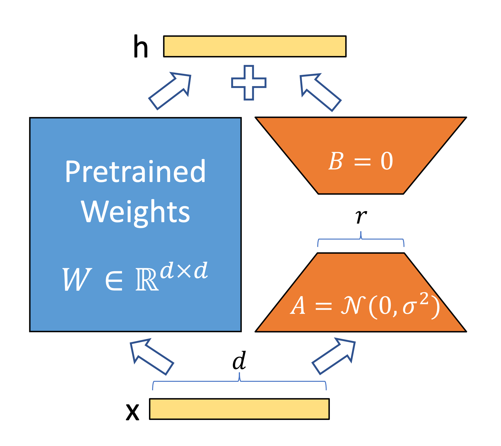
peft_model = get_peft_model(original_model, lora_config)r=32(Rank): This is the rank of the LoRA update matrices. It determines the size of the small adapter matrices. Essentially, for each weight matrix we’re adapting, LoRA will create two smaller matrices of size(original_dim, r)and(r, original_dim)instead of modifying the original(original_dim, original_dim)weight directly. For context, if a weight is 2048x2048, a full update is ~4 million parameters, whereas a LoRA adapter with r=32 is 2204832 ≈ 131k parameters – just ~3% of the original, since it has two small matrices.
lora_alpha=32: This is a scaling factor for the LoRA adapters. In many LoRA implementations, the actual update added to the model’s weights is scaled byalpha/r. By settingalpha = 32whiler = 32, the scale becomes 1.0 (32/32), meaning no additional scaling – the updates are taken as-is. Here we started with an scaling factor of 1.0, but essentially this is a hyperparameter to be tuned. Usually keepingalpha≥r.target_modules=['q_proj','k_proj','v_proj','dense']: This specifies which parts of the model will get LoRA adapters. Transformers models like LLaMA have many weight matrices in each layer. The notation here corresponds to:q_proj,k_proj,v_proj: the Query, Key, and Value projection matrices in the self-attention mechanism of each transformer block.dense: (likely the output projection of the attention or possibly the intermediate dense layer in the feed-forward network, depending on naming).
bias="none": This means we're not adding any trainable bias terms via LoRA, for simplicity.lora_dropout=0.05: A small dropout is applied to the activations within the LoRA adapters during training (5% dropout). This is a regularization measure to prevent overfitting on the new task, especially since the LoRA adapters are a relatively small number of parameters that could potentially overfit quickly.task_type="CAUSAL_LM": This tells the PEFT library what kind of model/task we are dealing with."CAUSAL_LM"means a causal language model (like GPT-style, predicting the next token given the previous tokens). This ensures that the LoRA implementation knows the architecture (for example, that we’re dealing with decoder-only blocks in a causal manner)
Training Setup: Small Batches, Accumulation, and Other Key Settings
Fine-tuning effectively with limited resources requires careful choice of training parameters. In the notebook, a TrainingArguments object (from Hugging Face Transformers) is created to specify how we train. These settings might look arcane at first, but each is chosen for a reason:
peft_training_args = TrainingArguments(
    output_dir = output_dir,
    warmup_steps = 1,
    per_device_train_batch_size = 1,
    gradient_accumulation_steps = 4,
    num_train_epochs = 1,
    learning_rate = 2e-4,
    optim = "paged_adamw_8bit",
    logging_steps = 25,
    save_steps = 25,
    eval_steps = 25,
    evaluation_strategy = "steps",
    do_eval = True,
    gradient_checkpointing = True,
    load_best_model_at_end = True,
    save_total_limit = 3,
    metric_for_best_model = "eval_loss",
    report_to = "none",
    group_by_length = True,
    dataloader_pin_memory = False,
    overwrite_output_dir = True,
)
Let's unpack the most important ones (some are straightforward, others deserve explanation):
Batch Size and Gradient Accumulation:
per_device_train_batch_size=1andgradient_accumulation_steps=4mean that although only 1 sample is processed at a time on the GPU, the optimizer will wait until 4 samples have been processed before updating the weights. Effectively, this simulates a batch size of 1×4 = 4 samples per update.Epochs and Warmup:
num_train_epochs=1– only one epoch (one full pass over the training dataset) is performed. Given the dataset size (the DialogSum dataset has a few thousand dialogues), one epoch with a decent learning rate can already improve the model, since we started from a pretty good pre-trained model. In other scenarios, you might do multiple epochs, but here it may have been enough, or it’s done for speed in a demo.warmup_steps=1is basically negligible learning rate warmup – essentially no warmup schedule (sometimes we do a few hundred steps of warmup in larger training runs to avoid shocking the model with a high learning rate at start, but here 1 step is nothing, meaning we ramp up to full learning rate almost immediately).Learning Rate:
learning_rate=2e-4(0.0002). This is relatively high for fine-tuning (often you see 1e-5 to 1e-4 for full-model fine-tuning). The companion theory article notes that finding the right learning rate is important – too low and the model won’t adapt enough, too high and training may diverge. This hyperparameter may be a good candidate for exploring furtherOptimizer:
optim="paged_adamw_8bit". This is an 8-bit AdamW optimizer provided by the bitsandbytes library. It means the optimizer states (like the moment estimates in Adam) are kept in 8-bit precision, further saving memory. "Paged" refers to a memory management strategy in bitsandbytes that handles large parameter sets by paging them in and out of memory efficiently. In short, this optimizer is almost equivalent to the standard AdamW (which is a good default for fine-tuning)Gradient Checkpointing:
gradient_checkpointing=True. We already enabled this on the model earlier, but this flag in TrainingArguments ensures the trainer is aware of it. This again helps keep memory usage in check during training at the cost of extra computation.
With training arguments defined, the notebook sets up an SFTTrainer (Supervised Fine-Tuning Trainer) from the trl library:
peft_trainer = SFTTrainer(
    model=peft_model,
    train_dataset=train_dataset,
    eval_dataset=eval_dataset,
    args=peft_training_args,
    tokenizer=tokenizer,
    data_collator=DataCollatorForCompletionOnlyLM(response_template_ids, tokenizer=tokenizer),
)
This is similar to Hugging Face’s Trainer, but tailored for scenarios like instruction tuning or chat fine-tuning. The key part to notice is the data collator: DataCollatorForCompletionOnlyLM. This collator is designed to prepare batches where we only compute loss on the completion part of the text. In our case, the "prompt" is the dialogue and the "completion" is the summary. We don't want the model to learn to predict the dialogue itself; we want it to predict the summary given the dialogue.
The notebook constructs a response_template which is basically a special token sequence that marks the beginning of the assistant's response. For example, it looks like "<|eot_id|><|start_header_id|>assistant<|end_header_id|>" in the code. These are special tokens indicating end-of-text and header tags. When this sequence appears, it signals that what follows is the assistant’s output (the summary).
Why is this needed? Imagine the training sample text is: Dialogue:
User: …
Assistant: ...
Summary: ...
We only want to train the model to generate the summary after seeing the dialogue. Without a special collator, the model would also be asked to predict the dialogue text (which it shouldn't have to, since the dialogue is given). By using this collator, we ensure the loss is only calculated on the summary part (the completion). This is a subtle but crucial detail in fine-tuning language models for tasks like Q&A or summarization – you always want to mask the context so the model doesn’t just trivially learn to copy inputs. The Hugging Face TRL docs linked in the notebook discuss this technique in more detail.
After training, the LoRA adapter can be saved with peft_model.save_pretrained(...) which the notebook does, allowing us to reuse this fine-tuned model later. The result is we have a model that, when given a dialogue, will (hopefully) produce a good summary of that dialogue.
Evaluation
After fine-tuning, it's important to evaluate how the model performs on data it hasn't seen (the test or validation set). In Notebook , they load the fine-tuned model (and also the original base model for comparison) and generate summaries for a set of dialogues. Then they compare those generated summaries to the reference (human-written) summaries using quantitative metrics.
The two main metrics used are ROUGE and BERTScore (and they also computed BLEU, another common metric, though we'll focus on ROUGE and BERTScore as requested). These metrics give us a sense of how close the model’s outputs are to the desired outputs.
Let's go through each metric to understand what they tell us:
ROUGE: Measuring Overlap with Reference Summaries
ROUGE stands for Recall-Oriented Understudy for Gisting Evaluation. It's a set of metrics commonly used to evaluate automatically generated summaries (and sometimes translations). The basic idea of ROUGE is to measure how much overlap there is between the model’s output and a reference output, in terms of n-grams (continuous sequences of tokens).
ROUGE-1: Overlap of unigrams (single words) between the generated summary and the reference summar
ROUGE-2: Overlap of bigrams (two-word sequences) between the generated and reference
ROUGE-L: Overlap based on the Longest Common Subsequence (LCS). his metric finds the longest sequence of words that appears in both the generated summary and the reference summary (not necessarily contiguously, but in order) and uses that to compute a score.
ROUGE mostly counts n-gram overlaps, which can miss the point in summaries that use different but valid phrasing—something common in dialogue. In this case, a metric like BERTScore may be more appropriate.
BERTScore: Measuring Semantic Similarity
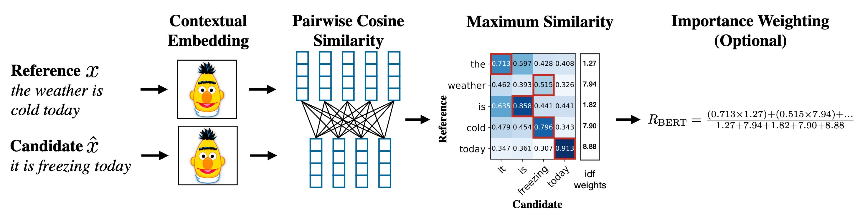
BERTScore is a newer metric that aims to address the weaknesses of ROUGE and BLEU by evaluating summaries (or translations) based on meaning rather than exact word overlap. Instead of looking for exact n-gram matches, BERTScore uses embeddings from a pre-trained model (like BERT or RoBERTa) to compare the generated text and the reference text.
The result is a score (or a set of scores P, R, F1) typically in the range 0 to 1, where higher means more semantically similar. A score of 1 would mean the two texts are essentially identical in meaning. In practice, you won't get 1 unless the text is exactly the same or a very close paraphrase. But BERTScore tends to give higher values than ROUGE for decent summaries because it rewards paraphrasing. For example, in our hypothetical "car" vs "automobile" case, BERTScore would likely consider "car" and "automobile" embeddings close, so it would give a high similarity for that part, whereas ROUGE-1 would have missed it.
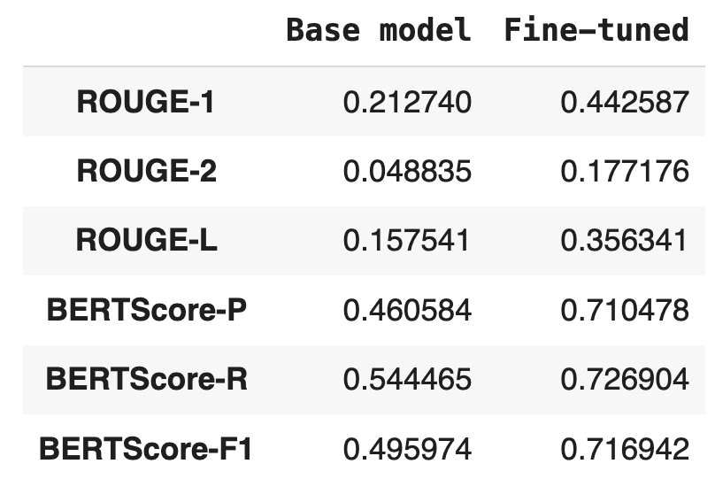
Results
After running the function calculate_metrics that uses the library evaluate from Hugging Face, the results demonstrate all metrics improved after fine tuning the model.
Conclusion
Through this walkthrough, we've connected the dots between the practical steps in the notebooks and the theoretical concepts of fine-tuning LLMs:
We saw how LoRA allows efficient fine-tuning by adding only a small number of trainable parameters (adapters) instead of updating the whole model. This aligns with the theory that large models have a lot of redundant capacity and a low-dimensional tweak (low-rank update) can often suffice to learn a new task.
We then talked about the evaluation metrics: ROUGE and BERTScore. ROUGE gives a sense of literal overlap (did the model say the important words?), while BERTScore measures semantic overlap (did the model capture the meaning?). Both are useful; together they give a fuller picture of summary quality.
By comparing the model before and after fine-tuning, we saw concrete evidence of improvement, which reinforces why fine-tuning is worth doing. The theoretical expectation was that tailoring a model to a task should improve performance – and the empirical results confirmed this, with ROUGE and BERTScore jumps.
We hope this post made fine-tuning clearer. Fine-tuning large language models involves a mix of clever ideas (like LoRA) and careful engineering (like managing training settings and evaluation). As you continue exploring, you can refer back to the companion theory post for more on why certain fine-tuning techniques are needed, and use this practical guide as a reference for how to implement them.
Next steps: You might try to replicate these results on a different dataset or with a different model. The good news is that with libraries like PEFT, the process will be very similar. You'd load a model, apply LoRA, pick reasonable hyperparameters, and train. Always keep an eye on both training loss and evaluation metrics to ensure your model is actually learning and not overfitting or diverging. And remember, metrics like ROUGE and BERTScore are there to guide you, but also qualitatively look at the generated outputs – sometimes a model might get a decent score but produce slightly off summaries. Combining human judgment with these metrics is the gold standard in evaluation.