Hyperparameter tuning with MLFlow and Optuna

Photo by Julia Koblitz on Unsplash

This article will explore the concepts of hyperparameter tuning through two powerful tools in Machine Learning: MLFlow and Optuna.

Hyperparameters are critical in determining the performance of a machine learning model. They control every aspect of model training and have a substantial impact on the model’s accuracy. However, finding the perfect set of hyperparameters is no simple task. Thankfully, tools like MLFlow and Optuna come into play to make our job easier.

MLFlow is an open-source platform that manages the entire machine learning lifecycle, including experimentation, reproducibility, and deployment. Optuna is an automatic hyperparameter optimization software framework, particularly designed for machine learning.

Whether you’re a seasoned data scientist or a beginner in the field of machine learning, this article will provide you with insights that can help make your machine learning models more efficient and accurate.

So, buckle up as we set out on this exciting journey of enhancing machine learning performance with MLFlow and Optuna!

Project structure

A typical Data Science project is composed of several parts. The diagram shows the steps of a data science project lifecycle, which is typically divided into two main phases: the data cycle and the model cycle.

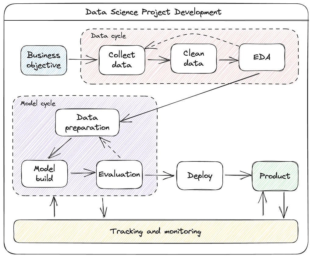
The data cycle starts with the business objective, which is the problem that the data science project is trying to solve. Once the business objective is clear, the next step is to collect data. This data can come from a variety of sources, such as internal databases, external datasets, or social media. Once the data is collected, it needs to be cleaned to remove any errors or inconsistencies.

The next step is to perform exploratory data analysis (EDA). This is where the data scientist will explore the data to gain insights into its distribution, patterns, and relationships. EDA can help the data scientist to identify the features that are most important for solving the business objective.

The model cycle starts with data preparation. This is where the data is pre-processed to make it ready for modeling. This can involve steps such as feature selection, dimensionality reduction, and normalization.

The next step is to build the model. This is where the data scientist will choose a machine learning algorithm and train it on the data. The goal is to create a model that can accurately predict the outcome of interest.

Once the model is built, it needs to be evaluated. This is where the data scientist will measure the performance of the model on a holdout dataset. The evaluation results will help the data scientist to decide whether the model is ready for deployment.

If the model is not performing well, the data scientist may need to go back to the data preparation or model building steps. Once the model is performing well, it can be deployed to production.

Tracking and monitoring is a component where the data scientist will track the performance from several experiments (model cycles). Also, this component is key to monitor the performance of the model in production and make adjustments as needed.

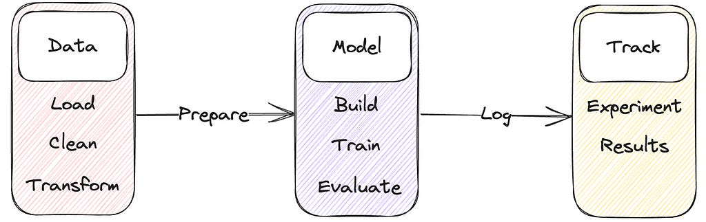
In this article we'll dive into part of this lifecycle: build a framework to load, process data, train a model and track experiments.

Data

This article uses a dataset to predict the quality of wine based on quantitative features like the wine’s “fixed acidity”, “pH”, “residual sugar”, and so on. This dataset is from UCI’s machine learning repository. For this example, I'm replicating MLFlow's tutorial (you can find it here).

Loading and cleaning

Since this dataset is clean and very well presented, we just need to load the data. Let's write a function to do so.

CSV_URL = "https://raw.githubusercontent.com/mlflow/mlflow/master/tests/datasets/winequality-red.csv"

def load_data() -> pd.DataFrame:
    try:
        data = pd.read_csv(CSV_URL, sep=";")
    except Exception as e:
        logger.exception(
            "Unable to download training & test CSV, "
            "check your internet connection. Error: %s", e
        )

    return data

There aren't missing values, so we don't need to do much about it.

<class 'pandas.core.frame.DataFrame'>
RangeIndex: 1599 entries, 0 to 1598
Data columns (total 12 columns):
 #   Column                Non-Null Count  Dtype  
---  ------                --------------  -----  
 0   fixed acidity         1599 non-null   float64
 1   volatile acidity      1599 non-null   float64
 2   citric acid           1599 non-null   float64
 3   residual sugar        1599 non-null   float64
 4   chlorides             1599 non-null   float64
 5   free sulfur dioxide   1599 non-null   float64
 6   total sulfur dioxide  1599 non-null   float64
 7   density               1599 non-null   float64
 8   pH                    1599 non-null   float64
 9   sulphates             1599 non-null   float64
 10  alcohol               1599 non-null   float64
 11  quality               1599 non-null   int64  
dtypes: float64(11), int64(1)
memory usage: 150.0 KB

I'm not going to focus on exploratory data analysis here, but you can take a peek into the statistics of the data.

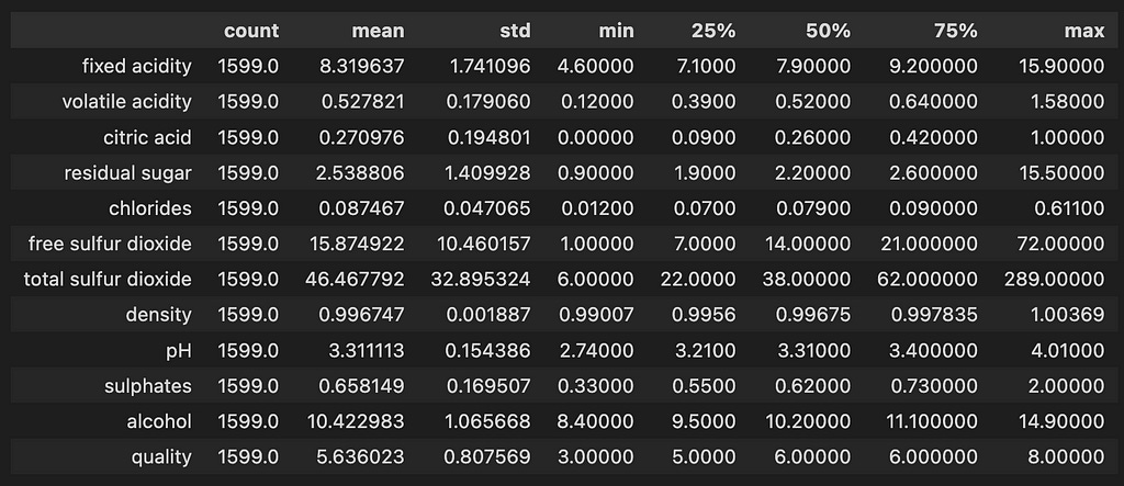
Prepare data

In an actual project, it would be required to standardize the features by applying normalization. Let's skip this step for now and focus on using Optuna and MLFlow for hyperparameter tuning.

We want to predict the quality of wine given several physicochemical properties. The values ranges from 3 .0 to 5.0 with standard deviation of 0.8. For this task, we'll build a linear regression model with the column quality being the target.

x = data.drop(["quality"], axis=1)
y = data[["quality"]]

What we need is to split our data into train and test. For this we'll use the well known train_test_split function from Scikit-learn. Our test set will have 25% of the whole dataset:

x_train, x_test, y_train, y_test = train_test_split(x, y, test_size=test_size)

Model

We'll be using ElasticNet from Scikit-learn. Elastic Net is a regularized regression method in scikit-learn that linearly combines both penalties, i.e. L1 and L2 of the Lasso and Ridge regression methods. It is useful when there are multiple correlated features. You can find a very good explanation about this model here.

We'll be performing a hyperparameter search with two parameters:

• alpha is the regularization parameter

• l1_ratio is the mixing parameter between the L1 and L2 penalties

Track

Now, let's set up our tracking framework. We'll use Optuna to do hyperparamether search and MLFlow to track each experiment. We'll use a callback from Optuna to send parameters and optimization metrics to MLFlow.

Before running our experiments, we have to start MLFlow server.

mlflow ui

After start the server, go to http://127.0.0.1:5000 , if everything is ok, you'll MLFlow's UI.

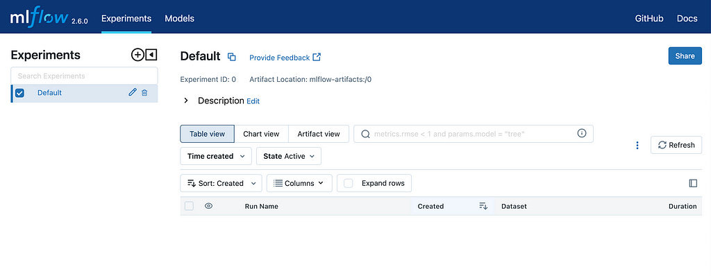
At this moment you don't have any experiments saved. You now have to set up the tracking URI.

import mlflow

mlflow.set_tracking_uri("http://127.0.0.1:5000")
tracking_uri = mlflow.get_tracking_uri()

Optuna has a callback to work with MLFLow, that allows logging parameters and objective results, let's set it up.

from optuna.integration.mlflow import MLflowCallback

mlflc = MLflowCallback(
    tracking_uri=tracking_uri,
    metric_name="rmse",
)

Train

Next step in our project is to finally train our model and perform the hyperparameter search. First, we need to create the objective function of our study

Since we'll be performing a search in alpha and l1_ratio we define those parameters with the method suggest_float from the trial object passed into the function objective at each trial.

@mlflc.track_in_mlflow()
def objective(trial: optuna.trial.Trial) -> float:
    """
    Optuna objective function for hyperparameter tuning of a regression model.

    Args:
        trial: An Optuna `Trial` object used to sample hyperparameters.
        x_train: A numpy array of shape `(n_samples, n_features)` containing
            the training data.
        y_train: A numpy array of shape `(n_samples,)` containing the target
            values for the training data.
        x_test: A numpy array of shape `(n_samples, n_features)` containing
            the test data.
        y_test: A numpy array of shape `(n_samples,)` containing the target
            values for the test data.

    Returns:
        The root mean squared error (RMSE) of the regression model on the test
            data.
    """
    params = {
        "alpha": trial.suggest_float("alpha", 0.05, 1.0, step=0.05),
        "l1_ratio": trial.suggest_float("l1_ratio", 0.05, 1.0, step=0.05),
    }
    model = ElasticNet(**params)
    model.fit(x_train, y_train)
    mlflow.sklearn.log_model(model, "model")
    y_pred = model.predict(x_test)
    rmse = np.sqrt(mean_squared_error(y_test, y_pred))

    return rmse

Note that we are using the decorator track_in_mlflow from the callback we set up before. This decorator enables the extension of MLflow logging provided by the callback. All information logged in the decorated objective function will be added to the MLflow run for the trial created by the callback.

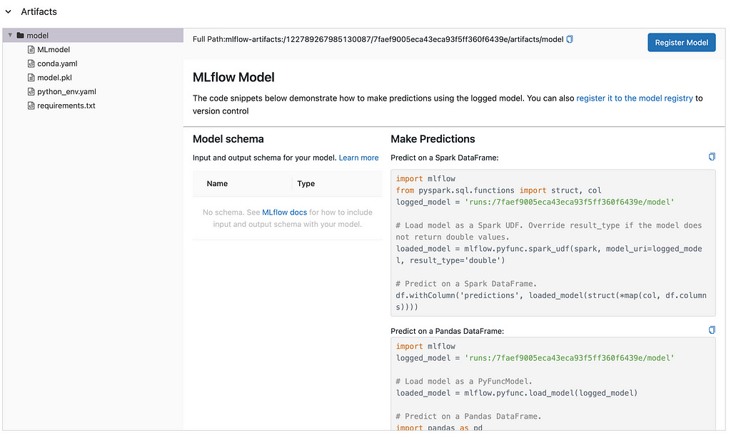
By including the function mlflow.sklearn.log_model inside our objective function, we can also log the model used and load them later if needed

That's it! Now you can run your study.

date_run = datetime.now().strftime("%Y%m%d_%H%M%S")
study = optuna.create_study(
    direction="minimize",
    study_name=f"elastic_net_{date_run}"
)
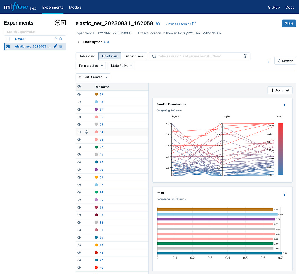
study.optimize(objective, n_trials=100, callbacks=[mlflc])

We can now go back to the MLFlow UI and explor the best performing model.

Since we're also logging models, we can see the information about any model from any experiment.

This is it! You built a hyperparameter search framework using MLFlow and Optuna. The notebook with this implementation can be found here.